

TypeSafe AI recently released Jev, a model that promises low latency (TypeSafe reports 70 to 500 ms per call) and inference so cheap that output tokens are not metered[1][2]. At the same time, TypeSafe says Jev “achieves similar levels of intelligence on System One tasks compared to existing LLMs”[1]. This is fascinating.
A claim like this raises some natural questions. How does it work: what is the architecture, and how does it differ from the typical autoregressive model? What are the key tradeoffs, and when does it make sense to use a model like Jev? Can I build, train or use one for my own use cases, and what does performance look like?
This article works through those questions in order: how Jev and models like it work, experiments I ran on open Qwen models to test the idea, and what we know about Jev itself.
An interactive version of this post is on my website here.
How decision models like Jev work
Jev is a “System One” model (the name echoes Kahneman’s System 1, fast intuitive judgement) from TypeSafe AI, described as “a frontier-intelligence function call: unstructured state in, typed probabilistic decisions out”[1]
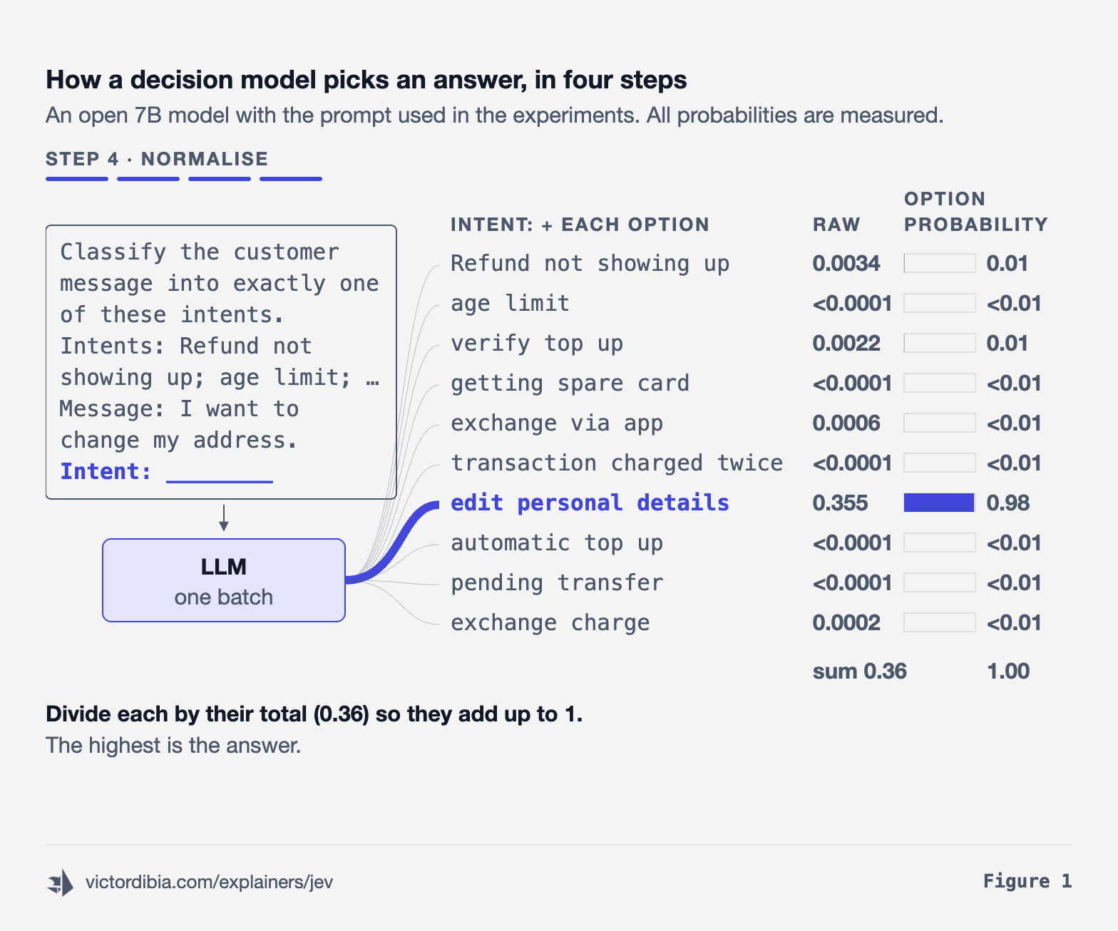
Models like Jev provide output in four steps:
Start with a decision. Given a state (the text the decision is about) and a list of options, pick one. For example: a customer writes to a bank, “I want to change my address.”, and we need to pick their intent from a list of 10 potential intents.
Turn it into a sentence to complete. Write a prompt that lists the options and ends exactly where the answer goes:
Classify the customer message into exactly one of these intents.
Intents: Refund not showing up; age limit; edit personal details; ... (10 in all)

Message: I want to change my address.
Intent: ___
Score every option. Append each option to the prompt and ask the model how likely that exact text is as the completion (the product of the probabilities of its tokens, the word pieces a model reads and writes). The options are known in advance, so nothing is generated, and all of them are scored in parallel. We call this step scoring: reading the model’s probabilities for text we supply, instead of generating text.
Normalise. Divide these probabilities by their total so they add up to 1. The results are the option probabilities, and the highest is the answer.
Jev packages this as an API with a few distinctive traits:
No text generation. “System One models do not write replies, produce code, or generate explanations of their reasoning”[7].
Many questions, one read of the input. The model “processes the state once and evaluates all questions against it in parallel”[2].
Three question types, all lists. A choice picks one of up to 255 options[8]. A score rates the state on 2 to 10 ordered levels[9]; I call it the rating-scale question, because “scoring” already means step 3. A noul (”short for bernoulli”[10]) answers yes or no with one probability.
Fast and cheap. TypeSafe reports 70 to 500 ms per call, against 3 to 329 s for frontier large language models (LLMs) on the same tasks[1], and charges $0.042 per million input tokens with output free[2].
Note: TypeSafe has not disclosed how Jev is implemented, but are likely to follow as similar approach above.
Calibrated decision models
While Jev is one implementation, we can think of this class of models as calibrated decision models. Decision means the goal is to select from a list of options, not to generate text. Calibrated refers to the model’s confidence, the probability it gives to the option it chose. A model is calibrated when its confidence matches its accuracy: if it gives a thousand answers at 90% confidence, about 900 of them are right.
In my opinion, confidence is important here because it lets us build systems and apps that do something ML models are notoriously bad at: say “I don’t know” or “I’m not sure” when confidence is low.
The avid reader is likely getting suspicious here: calibration is a hard problem. Early evidence suggests Jev is well calibrated. One independent benchmark measured its expected calibration error (ECE) at 0.0588 on 662 prompt-injection messages[12], meaning its confidence and its accuracy differed by about 6 percentage points on average. A stock model came close on the same task, as What we know about Jev shows.
Use cases for decision models
Decision models have a few properties that make them useful in production. First, the model can only select from a provided list of options, which removes a whole class of hallucinations and parsing failures: there is no answer that is not one of your options. Second, when the model is well calibrated, its confidence lets you build more thoughtful experiences that reflect certainty/confidence. The system can act when it is sure, ask a clarifying question when it is not, or hand off to a human. Third, it is fast and cheap enough to call on every step of a workflow, not just occasionally.
All of this suits tasks with structured output, and many production processes have that shape. A decision model fits when:
The answer can be listed: a category, an action, a yes or no, a level on a scale.
The decision is frequent or on the hot path, so latency and cost matter.
One judgement is enough. Everything happens in one pass, so tasks that need step-by-step reasoning are a poor fit; TypeSafe lists arithmetic and counting among Jev’s weak spots[13].
You can check the confidence against labelled examples from your own task.
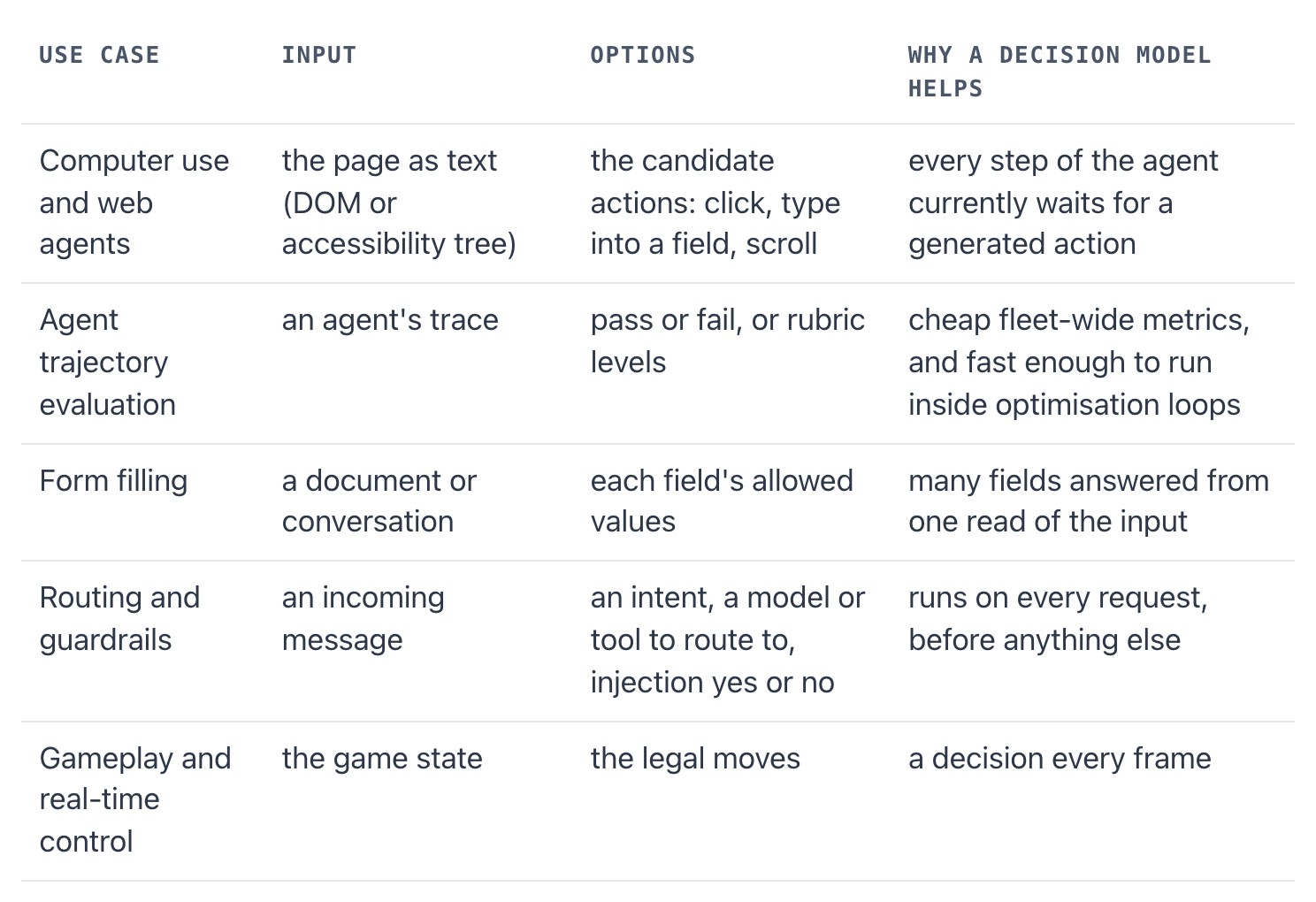
Computer use. In the computer-use chapter of my book, Designing Multi-Agent Systems[14], latency and cost are two challenges I highlight: complex tasks need many model calls, one per action, so delays and costs compound. One of the mitigations the chapter points to is smaller, faster models tuned for interface understanding and action prediction. A decision model fits that description: it reads the state of the page and selects the next action from the list of possible actions. Jev takes text only[2], so here the state would be the page’s text rather than a screenshot.
Agent evaluation. Teams running agents need both fleet-wide metrics and task-specific ones, and observability platforms need to score agents quickly. Evaluation matters even more inside optimisation loops, where an evaluator is called thousands of times, and a fast yes/no or rating-scale question is a good fit for both.
The one caveat is evaluation of the decision model itself. We need evals that tell us not just whether it is accurate, but whether it is calibrated, measured on labelled examples. The experiments below show why: accuracy can look fine while the confidence is badly off.
Why scoring is fast
To see why scoring works, and why it is fast, we first need to look at how a language model produces text.
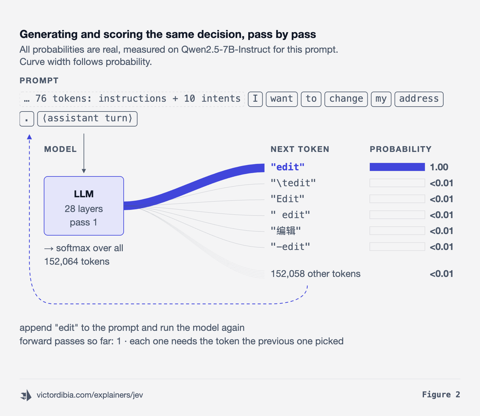
An autoregressive model takes text in and produces text out. The input is split into tokens, pieces of text such as a word or part of a word, from a fixed vocabulary (152,064 of them for Qwen2.5-7B, used later[15]). Each token becomes a vector, and the vectors pass through a stack of identical layers. After the last layer, every position is turned into one number per vocabulary entry, and a softmax turns those numbers into probabilities: the model’s prediction of the next token. One run of the input through all the layers is a forward pass.
One forward pass produces a next-token probability distribution at every position of the input, all at once.
There are two ways to turn those probabilities into a decision: generate the answer, or score the options.
Generating a decision
To generate text, we run a loop around the model: run a forward pass, pick a token from the distribution at the last position, append it to the input, and repeat until the model produces a stop token. There are two ways to get a decision this way:
Generate a label. Ask for the answer. The model generates a few tokens, for example
edit personal details, and you match that text to one of your options.Generate probabilities. Ask for a JSON object with a probability for each option. The model generates it token by token: every option name and every number.
This loop is serial and hence slow: each forward pass needs the token the previous one picked, so the passes cannot run at the same time. Modern models make each pass cheaper, mainly with a KV cache, which stores the work already done on earlier tokens so that each pass only processes the one new token. But the passes still run one after another. A short label takes only a few generation steps, while a probability for every option takes one step per token of the whole answer. Both also depend on the model behaving: a generated label can match no option, and generated JSON may not parse.
Scoring a decision
The model first reads the prompt: one forward pass over all its tokens, which also fills the KV cache. Unlike generation, this pass runs in parallel, because every token of the prompt is known before we start. Scoring relies on the same fact: the options are known in advance too. A second forward pass reads every option side by side, each one reading the cached prompt, and normalising their probabilities gives the answer. That is two passes, however long the options are, and scoring cannot return anything off the list, because you supplied the text of every option.
What scoring gives up
Options are judged separately. Each option is scored on its own, and one option cannot see another. The model never compares edit personal details with transaction charged twice directly; the comparison happens only when we normalise.
Different wordings compete. A score is the probability of a piece of text, not of an answer being right. In Figure 1, the model split its first word between “Edit” and “edit”, and only one of them is counted[16]. Word options the way the model would say them.
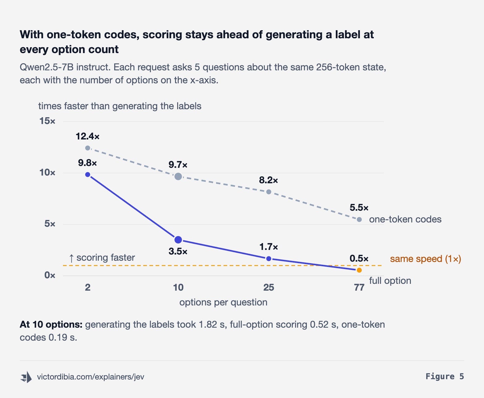
Cost grows with the number of options. Scoring reads every token of every option, so its cost grows with questions × options. A generated label costs about the same however many options there are: the model compares the options inside one forward pass and generates only the winner. Giving each option a one-token code, such as a letter, and reading only that avoids the second pass[3][4]; Can a cheaper readout do as well? measures what it costs.
Experiments with Qwen2.5 1.5B and 7B
To test all of this, I ran quick experiments on Modal using open Qwen2.5 models. The goal was not the fastest possible numbers, but to compare the approaches under identical conditions and report what we see and the conditions under which we see it[5].
Models: Qwen2.5 1.5B and 7B[15], each as a base model (trained only to predict the next token) and an instruct model (further trained to follow instructions and chat, the kind most APIs serve).
Hardware and software: one NVIDIA A10G GPU on Modal, Hugging Face transformers 4.46.3, 16-bit weights, one request at a time. No serving engine such as vLLM, which would make generation faster but add its own variables.
Scoring code: my own script, implementing the two passes described in Scoring a decision. An option’s option score is the sum of its tokens’ log-probabilities (the log of their product), and normalising the scores gives the option probabilities. I checked it against a slow version that recomputes the prompt for every option, on a 0.5B model; the two agreed to within 0.00003 in 32-bit arithmetic, and in the 16-bit arithmetic used for the runs they picked the same answer.
Data: for the intent question, 1,200 Banking77 test messages, sampled with a fixed seed, with 2, 10, 25 or 77 options (for fewer than 77, the correct intent plus randomly chosen wrong ones)[17]. For a yes/no question, “is this message a prompt injection?”, all 662 messages of the deepset prompt-injections dataset[18].
Cost: about $4 of GPU time across every run, as billed by Modal. The code, the raw results and a cost ledger are in the site’s repository.
Is scoring faster than generation?
On the 7B instruct model, reading a 339-token prompt took 0.115 s, and each generated token added 36.9 ms. A generated label (11 tokens) took 0.47 s, and generated probabilities for 10 options (125 tokens) took 4.57 s. Scoring the same question took 0.23 s.
In every setting where generated probabilities were run, scoring was 7× to 54× faster than generating probabilities on the 7B, and 13× to 132× on the 1.5B. With 77 options, generated probabilities would be about 890 tokens, roughly 33 s on the 7B by the fitted line (not run).
Against generating a single label, the answer depends on the number of options, the trade-off from What scoring gives up. With 5 questions about the same state on the 7B, scoring was 9.8× faster at 2 options, 3.5× at 10 and 1.7× at 25, and at 77 options it was slower (0.5×). A longer state narrows the gap too: 3.5× at 256 state tokens, 2.6× at 1,024 and 1.4× at 4,096, because processing the state starts to dominate.
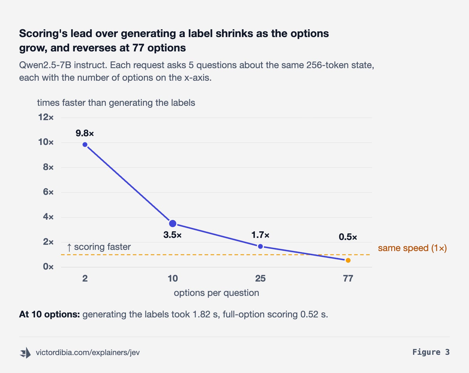
Part of the slowdown at many options comes from our setup, not the technique. Our code makes a copy of the prompt’s KV cache for every option before reading it; serving engines such as vLLM share a single copy, so they would move the break-even point to more options. A serving engine would also make generation several times faster, so all the speedups here are upper bounds. Either way, every token of every option still has to be read, so scoring’s cost keeps growing with the number of options. More questions about the same state, by contrast, are cheap: the state is read once, and each question only adds its own options.
Is scoring as accurate as generation?
Scoring was at least as accurate as generating a label.
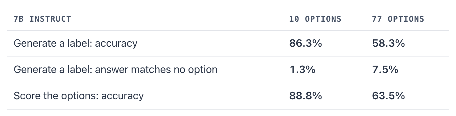
At 10 options the two approaches picked the same answer on 98.5% of messages. Generated labels were measured on a subset of 400 messages, scoring on all 1,200. Model size matters more than the approach: at 77 options, scoring was right 39% of the time with the 1.5B instruct model and 64% with the 7B.
Are the models calibrated?
Base models were close to calibrated; instruct models were not. At 10 options, the base models’ ECE was 0.05 (1.5B) and 0.02 (7B), while the instruct models’ was 0.18 and 0.10. Scale helped but did not fix it: at 77 options, the 7B instruct model’s average confidence was 95%, and it was right 64% of the time. The base models go against earlier findings that neural networks and language models are poorly calibrated[19][20]; the instruct models agree with them, and match what OpenAI reported for GPT-4: well calibrated after pretraining, and significantly less so after the post-training that turns it into a chat model[21].
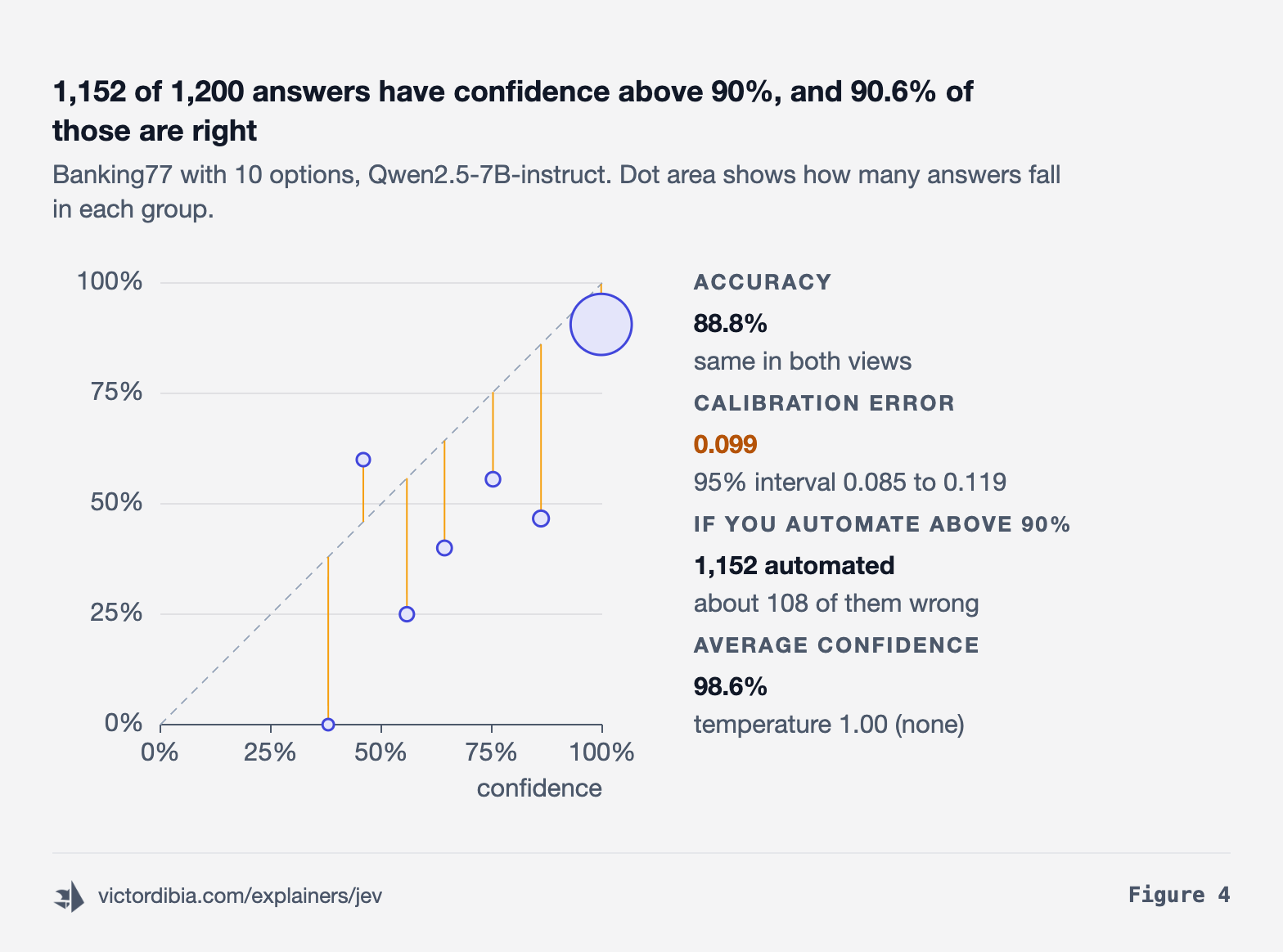
Figure 4 shows where the instruct model goes wrong. We sort its answers into groups by confidence and compare each group’s average confidence with the fraction that were right, which gives a reliability diagram; a calibrated model sits on the diagonal. The instruct model puts 1,152 of its 1,200 answers above 90% confidence, at an average confidence of 99.8%, and only 90.6% of those are right.
Calibrating with temperature scaling
Temperature scaling divides every option score by one fitted number, the temperature, before normalising. It never changes which option wins, so accuracy stays the same, but it spreads the confidence out. Fitted on 600 labelled messages and tested on the other 600, it brought the 7B instruct model’s ECE from 0.10 to 0.03, about as good as the 7B base model (0.02). Because it keeps the order, it only moves where the 90% line falls. Before scaling, about 108 of the answers above 90% were wrong; after, about 23. The catch is that it needs labelled examples from your own task.
One more choice affects calibration: how an option’s tokens are combined into a score. Averaging their log-probabilities instead of summing them made the 7B base model underconfident (44% average confidence, 85% right), while summing made the instruct model overconfident. Pick one way of computing the score, and calibrate that one.
What about generating the probabilities directly?
Asking the model to generate its probabilities as JSON was the worst approach we measured. At 10 options, 32% of the 1.5B’s outputs and 7% of the 7B’s were not valid JSON. On the outputs that did parse, the 7B was right 84.1% of the time, against 86.3% for a generated label and 88.8% for scoring, and its ECE was 0.13, against 0.10 for raw scores. It was also the slowest.
Can a cheaper readout do as well?
Full-option scoring pays for every token of every option (What scoring gives up), yet on the running example almost all the difference between options sits in the first token: once the model has produced “edit”, the rest of edit personal details is close to certain (0.999 and 1.000), because it is copying from the list in the prompt. A cheaper readout, used by the open reproductions[3][4], lists the options with a letter each (A, B, C, and two-letter codes past 26) and reads the probability of each letter at the answer position. Each code is one token, so a single forward pass gives a probability for every option, however many there are. Fine-tuned letter classifiers, such as the one in Together AI’s tutorial, generate the letter instead[22]; on the 7B instruct model the generated letter matched the readout’s top letter on 99.5% of messages.
I ran the letter readout on the same messages, options and order as the full-option scorer, so every difference below is measured on the same items.
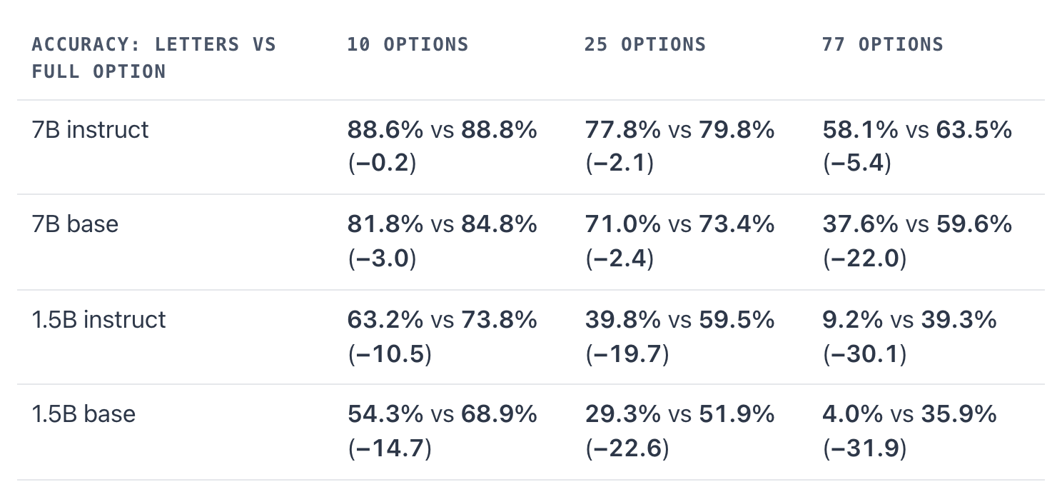
On the 7B instruct model, letters were within about two points of full-option scoring up to 25 options, and 5.4 points behind at 77. The 7B base model kept up to 25 options but was 22.0 points behind at 77, the 1.5B instruct model fell well behind above two options, and the 1.5B base model at every count. Mapping a letter back to its meaning is a task in itself, and small models do it poorly. The 1.5B base model also showed position bias: with two options it picked A 87% of the time, when A was right 52% of the time. Calibration was not the problem. After temperature scaling, the 7B instruct model’s ECE at 10 options was 0.028 with letters and 0.028 with full options.
The gain is in cost. With the state shared across questions, reading the letters for 20 questions of 77 options took 0.54 s on the 7B, against 13.6 s for full-option scoring. For a single question, reading the letters costs about one pass over the prompt (0.14 s at 10 options), and generating the letter instead adds one more step (0.17 s).
Is a calibrated model always useful?
No. Calibration says the confidence matches how often the model is right. It says nothing about how often the model is confident. A calibrated model that knows little gives low-confidence answers most of the time (near 50% on a yes/no question), and almost none of them clear a 90% bar.
Take the yes/no question “is this a prompt injection?”, asked of all 662 messages. The 1.5B instruct model had an ECE of 0.04 after scaling, and an accuracy of 62.8%, against 60% for always answering “not an injection”. (For yes/no questions I used Platt scaling, which fits two numbers instead of one.) The 7B instruct model reached 93.0% when the prompt said what the assistant is for.
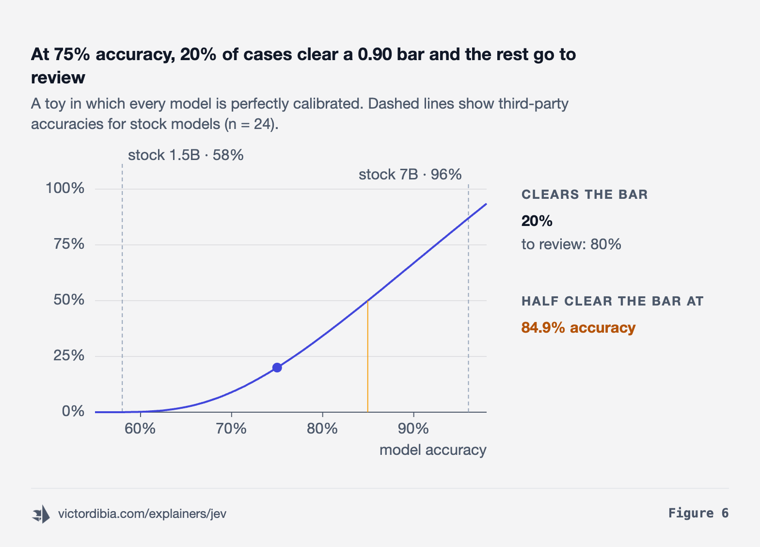
So judge a decision model by how many cases clear your bar, and set the bar from your costs.
What we know about Jev
TypeSafe has said little about how Jev works. When asked on Hacker News, their CEO described the architecture as “close to the chest for now”, and made only one statement about the mechanism: “strings (and all sequential data structures) are not allowed at all - this is how we make sure all outputs can be computed in parallel”[10]. That rules out generation, and it is why I think Jev is most likely a form of scoring: a model that reads probabilities for a fixed set of options instead of writing an answer.
What TypeSafe does say is that Jev is trained to be calibrated, using a method they call Reinforcement Learning for Calibrated Decisions (RLCD), aimed at “answers with epistemically honest probabilities”[1]. The method has not been published. Scoring any model gives you speed and answers that are always on the list, but an instruct model’s confidence needs extra work before you can trust it: training for calibration, as TypeSafe says they did with RLCD, or labelled examples from your own task, as temperature scaling needed in our experiments. It is also the part TypeSafe has published the least about. They publish no reliability diagram or ECE[23], and their one accuracy-by-confidence number is 27 of 30 answers correct above 0.9 confidence, on an older model, which leaves a wide 95% interval (74% to 97%)[24]. Their own benchmark also scores Jev against labels “generated via an average of the responses of GPT-6 Astra and Claude Fable 5.1”[23], so its accuracy numbers tell us how often Jev agrees with those two models, not how often it is right.
The best outside evidence comes from a third party who ran Jev on the same 662 prompt-injection messages we used[12]. With the task described in the prompt, they measured 96.5% accuracy and the 0.0588 ECE mentioned earlier; without it, 89.7% and 0.0928. Our stock 7B instruct model, with no special training, reached 93.0% with an ECE of 0.061, and 86.9% without the task description[5]. The prompts differ and the measurements were made by different people, so I would read this as indicative only. Still, it suggests a stock model gets within a few points of Jev’s accuracy on this task, with similar raw calibration.
One question stays open: whether Jev reads every option in full, as our scorer does, or reads all of them from one position, like the letter readout. Two details point to the second: choices are capped at 255 options, and TypeSafe’s launch post says that past the cap Jev falls back to “scoring independently then making an explicit choice”[1]. Timing requests from 2 to 255 options would be strong evidence: if latency stays flat, Jev reads one position per question.
Conclusion
In this article, we looked at how decision models like Jev work, in four steps: start with a decision, represent it as a sentence to complete, score the probability of each option, and normalise the results into a probability for every option. Ideally those probabilities are calibrated, so the confidence can be trusted.
We then tested the idea on open Qwen2.5 models. Scoring was 7× to 54× faster than generating the probabilities, and about 9.8× faster than generating a label with 2 options (7B model, 5 questions). Its lead shrinks as the options grow, and on the 7B at 77 options it was slower, unless each option gets a one-token code, which kept scoring ahead at every option count with little loss of accuracy on the 7B model.
Calibration turned out to matter as much as speed. Base models were close to calibrated, but instruct models were overconfident: at 77 options, the 7B instruct model’s average confidence was 95%, while it was right 64% of the time. Temperature scaling fixed most of that, but it needs labelled data, and this is also where training for calibration, as TypeSafe says it does for Jev, could help.
If you want to build on this, the sequence I would follow is:
Build an eval set from your own task, in the same sentence-completion format, with labelled answers.
Measure accuracy and calibration, not just accuracy: a reliability diagram and ECE on that set.
Fix what the measurements show: temperature scaling if the confidence is off and you have labels, fine-tuning if accuracy is too low, and one-token codes if you have many options and need speed.
Set the confidence threshold from your costs, and send everything below it to a person or a follow-up question.
No Jev API calls were made for this article. If you have tried Jev or built something similar, tell me what breaks.
References
TypeSafe AI (2026). Introducing System One Models & Jev (accessed 2026-09-19)
TypeSafe AI (2026). TypeSafe docs: Models (jev-1.13.0 price, limits, text-only input) (accessed 2026-09-19)
rorshopping (2026). jev-on-a-laptop at commit 5821d91: typed decisions on stock 1.5B-8B models, 16 GB M5 MacBook Air (third-party measurement) (accessed 2026-09-19)
Victor Dibia (2026). Measurements made for this page, 2026-09-20: our own option scorer on Qwen2.5 1.5B and 7B (base and instruct), one NVIDIA A10G on Modal, 16-bit weights, Hugging Face transformers 4.46.3, one request at a time, median of 3-10 repeats after 2 warmups. Code, raw JSON and a generated summary are in the site repository under docs/explainers/jev/experiments/modal_lab
TypeSafe AI (2026). TypeSafe docs: System One (accessed 2026-09-19)
TypeSafe AI (2026). TypeSafe docs: Choice (accessed 2026-09-19)
TypeSafe AI (2026). TypeSafe docs: Score (accessed 2026-09-19)
TypeSafe AI CEO, via Hacker News (2026). Hacker News thread ‘Introducing System One Models and Jev’, comments by user CompleteSkeptic (’CEO here’): ids 49719122 (no sequential outputs), 49718824 (architecture), 49718407 (noul = bernoulli) (accessed 2026-09-19)
Gaurav-Gosain (2026). jev-sec-bench at commit fdb16b9: Jev on the 662 deepset prompt-injection messages, with calibration error (third-party measurement) (accessed 2026-09-19)
TypeSafe AI (2026). TypeSafe docs: Known limitations of jev-1.13 (accessed 2026-09-19)
Victor Dibia (2026). Designing Multi-Agent Systems, Chapter 5: Building Computer Use Agents (action generation, interface representation, action execution)
Qwen team, Alibaba Cloud (2024). Qwen2.5-7B-Instruct model card and config.json: 28 layers, hidden size 3,584, 28 attention heads, 4 key-value heads, vocabulary 152,064, 32,768-token context (accessed 2026-09-20)
Holtzman, West, Shwartz, Choi & Zettlemoyer (2021). Surface Form Competition: Why the Highest Probability Answer Isn’t Always Right (’different surface forms compete for probability mass, even if they represent the same underlying concept’)
deepset (2023). deepset/prompt-injections: 662 messages, 263 labelled as injections (accessed 2026-09-20)
Guo, Pleiss, Sun & Weinberger (2017). On Calibration of Modern Neural Networks (’modern neural networks, unlike those from a decade ago, are poorly calibrated’; temperature scaling ‘is surprisingly effective’)
TypeSafe AI (2026). TypeSafe workflow evals (accessed 2026-09-19)
TypeSafe AI (2026). TypeSafe cookbook: Classification using confidence (60 SEC filings, 75 groups, jev-1.12) (accessed 2026-09-19)